Please note this text assumes you have some basic Mathematical knowledges concerning functions. Of course you can apply the formulaes without knowing what continuity or derivability is, but i think it should be most valuable to learn what they are for computer works.
Also note that this text is aimed at assembly language programming (though one
can use another language) and integer arithmetic, because this is the only way
to go fast with small expense of transitors (like in my lovely ARM processor).
Suppose you're programming something that requires loads of processing time, like a synthesis sample (1d) or a raytracer (2d)... But you would like it to run faster, even if you must have a lesser quality. A standard method to speed things up is to perform the precise computation on less points, and to add extra values with linear interpolation.
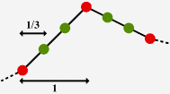
| Let's see how we proceed for when dimension is 1, as shown in "linear.gif". The red points are the one computed with the precise (and heavy) algorithm, and the green ones are added afterhand with a linear interpolation. |
|
In our example, if red points' heights are called h0; h1 and h2, the heights of green points will be (2*h0+h1)/3; (h0+2*h1)/3; (2*h1+h2)/3 and (h1+2*h2)/3. This values were found by calculating the equation of the line (hence the name linear interpolation) passing by (0;h0) and (1;h1), which is h(x)=h0+x*(h1-h0), and computing h(1/3); h(2/3). The same was done on the second segment.
As usual, if we take a power of two for the denominator of the x values, things will be much easier and the interpolations will need additions only since we'll use fixed point arithmetics. If we want to add 2^p%-1 green points the code will look like this:
  ... Compute the precise edges in h%(j%) for j%=1 to n% ...
        x%=0
        FOR j%=0 TO n%-1
          h%=h%(j%)
          dh%=h%(j%+1)-h%       :REM (h(1)-h(0)/2^p%) <<p%
          h%=h%<<p%             :REM Convert h0 to fixed point
          FOR i%=0 TO 2^p%-1
            POINT x%,h%>>p%
            x%+=1
            h%+=dh%             :REM h+=h(1)-h(0)/2^p%
          NEXT i%
        NEXT j%
A better version would probably make some rounding before plotting the point. But all this sounds nice and fast, isn't it?
Hummm! Fast it sure is, but nice... It depends upon what you are doing.
Many demos feature the standard tunnel effect, and they use this technique by
performing "raytracing" on a small 41*33 grid and then enlarging the values
with bichannel (they need two coords u;v to acces the map) bilinear (because
we interpolate on x and y for each block) interpolation on 8*8 blocks. In this
case the result is ok, but it won't always be so, especially when you have
quickly changing values (when you enlarge a raytraced image?).
The idea is to use a better interpolation function. In this chapter we'll use a cubic (ie of degree 3) polynomial, and the difference is stunning.
For explanation purposes, we'll assume from now on that we are in dimension 1, and that h(0);...;h(n) are our original points. Our aim is to replace each segment [h(i);h(i+1)], by a function fi(x)=ai*x3+bi*x2+ci*x+di so that fi(0)=h(i) and fi(1)=h(i+1) (note that i will be in [1;n-1]).
Obviously, we have 4 parameters (ai;bi;ci and di), and only 2 conditions, so we can set up two more conditions. As you can see, the linear interpolation produces sharp edges on the original points, and this is what we want to get rid off, isn't it?
Some mathematics would tell us that a sufficient condition to have a regular curve, without those sharp edges, is that the derivative of the function (exists and ;) is continuous. So we'll try to set up 2 more conditions on the derivatives, so that the slope on the left of h(i) is the same as the one on its right (which is obviously not the case with linear interpolation). All the work was to find those conditions, and here they are:
| In "cubic1.gif", you can see the original points in red and the tangents as red segments, which always are parallel to the grey dotted segments joining h(i-1) and h(i+1). Thus we can conclude that the derivative for each point is (h(i+1)-h(i-1))/2 (we divide by 2 because i+1 and i-1 are distant of 2). | 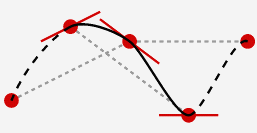
|
So, now we have 4 conditions for the function fi(x)=ai*x3+bi*x2+ci*x+di:
        fi(0)=h(i)
        fi(1)=h(i+1)
        fi'(0)=(h(i+1)-h(i-1))/2
        fi'(1)=(h(i+2)-h(i))/2
With some calculii, and knowing that fi'(x)=3*ai*x2+2*bi*x+ci, we find:
        di=h(i)
        ci=(h(i+1)-h(i-1))/2
        bi=(-h(i+2)+4*h(i+1)-5*h(i)+2*h(i-1))/2
        ai=(h(i+2)-3*h(i+1)+3*h(i)-h(i-1))/2
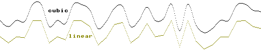
And now we have the whole function which is continuous, derivable and with a continuous derivative (because fi'(1)=fi+1'(0) etc...). And the resulting interpolation looks much better than a stupid linear one (see "cubic2.gif").
Ok, now moving on the hard subject of the implementation in fixed point arithmetic (and assembly of course ;). First, go have a look at my article dealing with incremental square/cubes computation... Done? Ok, i assume you did. The four coefficients to compute all this incrementaly are:
        val=a0
        inc1=a3*h^3+a2*h^2+a1*h
        inc2=6*a3*h^3+2*a2*h^2
        inc3=6*a3*h^3
Of course for an assembly version you'll use h=1/2n and shifts instead of
divisions, as explained in the squares.txt article. The drawing loop will look
like the following:
        val+=inc1
        inc1+=inc2
        inc2+=inc3
        plot val
So you need 3 additions (and some shifts on processor that, unlike ARM, don't have shifts for free) and 4 registers to implement this one. Bigger and slower than linear interpolation, but worth the prize anyway i think.
Oh, btw, it can be mathematically proven (this is a classic when playing with
Bezier curve) that the curve is entirely contained in the convex polygon formed
by the points (i;h(i)); (i+1;h(i+1)) and by (i+1;h(i)+fi'(0)) and
(i;h(i+1)-fi'(1)). So to ensure the interpolated values stay in the choosen
range (probably [0;255]) you'll need to set conditions so that h(i)+fi'(0) and
h(i+1)-fi'(1) also are.
This one was much harder to do (fasten your seatbelt), but the base idea is the same, ie replace each segment by a function fi(x)=aix2+bi*x+ci of degree two. The gain lies in the implemenation which needs only two additions (only one more than linear!) and 2 (TWO!) registers under certain circumstances (yes, the same amount as for linear interpolation, probably only possible on ARM ;).
This time we need three conditions, since we have three parameters. As usual we'll have two conditions dealing with the extremities, and the choice is left to us for the third condition. Sounds a bit annoying to have only one extra condition, because we would like to control two derivatives, isn't it? (he, he, says the one who knows more! ;)
One could try something a bit different, like fi(0)=h(2*i), fi(1)=h(2*i+2) and fi(1/2)=h(2*i+1) which makes for three conditions, but this wouldn't allow a continuous derivative. And there could be more choices, but i only found one sensible choice which i will expose to you right now.
| We must have at most 3 control points (or 3 conditions), and to simplify a bit let's call them h0;h0.5 and h1 (in orange) and have a look at "quad1.gif". One can notice that with three points organised in this way (which is not the standard one, but more on this later), we could set the conditions so that the function goes through h0 and h1, and then both derivatives would only need h0.5 to be controlled. | 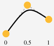
|
The derivative in h0 will be 2*(h0.5-h0) (we multiply by 2, ie divide by 1/2 because the distance is 1/2) and the one in h1 will be 2*(h1-h0.5), so we have:
        f(0)=h0
        f(1)=h1
        f'(0)=2*(h0.5-h0)
        f'(1)=2*(h1-h0.5)
Knowing that f(x)=a*x2+b*x+c, and so f'(x)=2*a*x+b, we can calculate:
        c=h0
        b=2*(h0.5-h0)
        a=h1-2*h0.5+h0
And you will admit that with such formulaes, we could easily compute the interpolated points between the [0;1] interval, again with the tricks explained in the article dealing with incremental squares/cubes computation.
| But in the original problem we were having segments defined by two points (in red) to replace with another interpolation function. For cubic interpolation it was quite easy to know which set of four points to take. But the symmetry of the problem don't seem to allow to take three points... I bypassed this problem by changing it a bit: instead of interpolating between [i;i+1], i worked in [i-0.5;i+0.5], thus changing the symmetry of the problem as shown in "quad2.gif". I needed two fake point i-0.5 and i+0.5 (orange), which i choosed so that h(i-0.5)=(h(i-1)+h(i))/2 and h(i+0.5)=(h(i)+h(i+1))/2. | 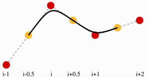
|
The unoptimised algorithm looks like this. You can improve it by developping
the expressions of a;b and c which depends only upon h(i-1); h(i) and h(i+1).
        FOR i=1 TO n-1

          REM Compute the three heights for quadratic interpolation
          y0=(h(i-1)+h(i))/2
          ym=h(i)               :REM Can't call it y0.5 or so
          y1=(h(i)+h(i+1))/2

          REM Compute the coefficients for quadratic interpolation
          c=y0
          b=2*(ym-y0)
          a=y1-2*ym+y0

          REM Compute the coefficients for incremental version
          value=c<<(2*m)
          inc1=a+(b<<m)
          inc2=a<<1

          REM Interpolate
          x=2^m*i
          FOR j=0 TO 2^m-1
            PLOT x,value>>(2*m)
            value+=inc1
            inc1+=inc2
            x+=1
          NEXTj

        NEXTi
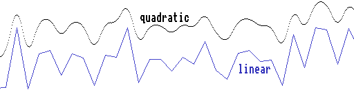
So, we have an easy way of computing quadratic interpolation, with only two additions per point, and by choosing m<=5 (ie at most 32 points interpolated) i was able to mix inc1 and inc2 in a single register. I must say the whole is really fast (provided you have an ARM and are programming in assembly ;) and very nice. In fact, i really doubt one can make the difference between cubic and quadratic interpolation visually. ("quad3.gif")
It also has an advantage. As for cubic interpolation, the interpolated
function will be completely enclosed in the triangle formed by the points
(i-0.5;(h(i-1)+h(i))/2); (i;h(i)) and (i+0.5;(h(i)+h(i+1))/2), and this tells
us that provided our original points h(i) are in the range [0;255], so will the
be the quadratic curve. No need to cope with more conditions as in cubic
interpolation. The inconvenient being that nothing ensures the original values
will be reached (and they probably won't be), so there's a kind of smooth
performed by the quadratic interpolation.
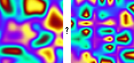
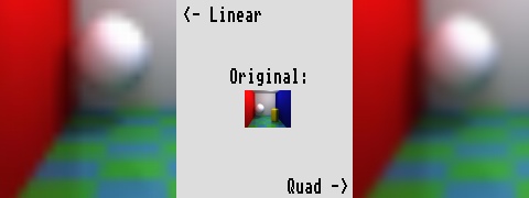
Ok, now have a look at both those images. The raytraced one must be viewed in 16 millions colors, or the rounding or dithering will spoil the effect. They both feature quadratic vs linear interpolation. We can see the standard linear interpolation artifacts (a value reached on one column/line only), and the difference leaves absolutely no chances to linear interpolation, except for some effects that won't require it because the model is regular enough (mapped tunnels for example).
I have not made much tests with cubic vs quadratic, because the difference is too small to be noticed visually. But the difference exists all the same. Ok, it will be a bit technical here.
Quadratic interpolation is made with polynomials of degree two, while cubic uses degree 3 polynomials. So the derivative of the quadratic functions will be a succession of connected segments (french mathematicians would tell the derivative is "affine par morceaux") while the derivative of the cubic interpolation will be composed of connected quadratic functions. Moreover this latter derivative function is itself derivable, and its derivative is continuous. To sum up we have:
This is not very important for visual appearance, but in case you want to take the derivative (or approximate it) with for example an emboss functions (bump mapping is not far away) you must take cubic interpolation to have something nice. Otherwise quadratic is more than effective.
Ok, i think i've said it all. You can have some ARM assembly source code for dim=1 quadratic interpolation here ("quad1.bas"), and if you want source for the dim=2 case, you can have it alongside my demo Wish You Were Beer. I hope to see quadratic interpolation more frequently in demos, because it's far better than linear one. And don't forget to credit/thank me in case you found this article valuable.